In Class Ex 6: Spatial Weights

Published

February 13, 2023

Modified

February 19, 2023

Setup

Install and load R packages

pacman::p_load(sf, tmap, sfdep, tidyverse)

Importing data

Aspatial data | Attribute table

As tibblr

hunan2012 <- read_csv("data/aspatial/Hunan_2012.csv")

Geospatial data

st_read( ) is an sf function. Import Hunan shapefile into R as an sf dataframe.

hunan <- st_read(dsn = "data/geospatial",
                 layer = "Hunan")

Reading layer `Hunan' from data source 
  `C:\zoe-chia\IS415\In-class_Ex\In-class_Ex06\data\geospatial' 
  using driver `ESRI Shapefile'
Simple feature collection with 88 features and 7 fields
Geometry type: POLYGON
Dimension:     XY
Bounding box:  xmin: 108.7831 ymin: 24.6342 xmax: 114.2544 ymax: 30.12812
Geodetic CRS:  WGS 84

Data cleaning

Combine both dataframes with left join

One is tibblr, one is sf, which has a geometric column. The left data frame should be the sf dataframe with geometric data.
We use the left_join function of dplyr. The function automatically joins by the common column, “County”.

Note

Make sure to check that the “County” columns in both dataframes have the same structure.

hunan_GDPPC <- left_join(hunan, hunan2012) %>%
  select(1:4, 7, 15)

Exploratory Data Analysis

Plotting Choropleth Map

tmap_mode('plot')
tm_shape(hunan_GDPPC) + 
  tm_fill("GDPPC", 
          style = "quantile", 
          palette = "Blues", 
          title = "GDPPC") + 
  tm_layout(main.title = "Distribution of GDP per capita by district, Hunan Province",
            main.title.position = "center",
            main.title.size = 0.8,
            legend.height = 0.30, 
            legend.width = 0.25,
            frame = TRUE)+ 
  tm_borders(lwd = 0.1,
             alpha = 0.6) + 
  tm_compass(type="8star", size = 2) + 
  tm_scale_bar() + 
  tm_grid(alpha = 0.2)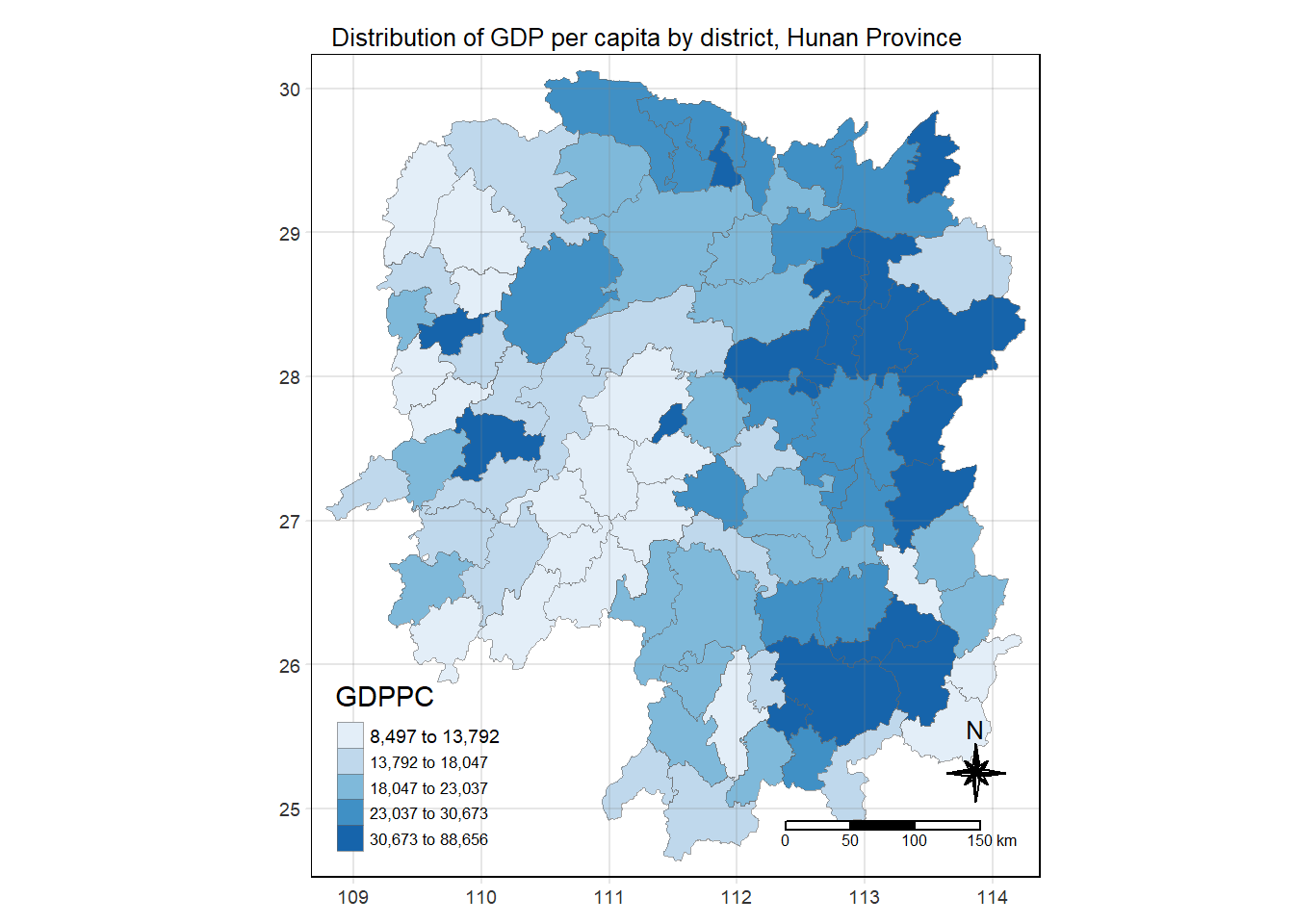

Identify Area (Polygon) Neighbours

Contiguity neighbours method

Queen’s Method

For sf format, st_contiguity() is used to derive a contiguity neighbour list by using Queen’s Method. Default is queen = TRUE.
For sp format, use spdep’s poly2nb() (polygon to neighbour) function.
dplyr’s mutate() creates a new field nb to store the result of st_contiguity
.before = 1 places the new field as the first column

cn_queen <- hunan_GDPPC %>% 
  mutate(nb = st_contiguity(geometry),
         .before = 1)

Rook’s Method

cn_rook <- hunan_GDPPC %>%
  mutate(nb=st_contiguity(geometry, queen = FALSE),
         .before = 1)

We now know it’s neighbours.

K-Nearest Neighbours

Computing contiguity weights

Distance based method

Contiguity weights: Queen’s Method

wm_q <- hunan_GDPPC %>%
  mutate(nb = st_contiguity(geometry),
         wt = st_weights(nb),
         .before = 1)

Contiguity weights: Rook’s Method

wm_r <- hunan_GDPPC %>%
  mutate(nb = st_contiguity(geometry, queen = FALSE),
         wt = st_weights(nb),
         .before = 1)

st_dist_band() lower limit always has to be 0