In-class Exercise 2: Geospatial Data Wrangling

Published

February 6, 2023

Load Packages and Data

sf: handle geospatial data
tidyverse: for data science work (data handling, manual processing and manipulation)
funModeling: quick exploratory data analysis

pacman::p_load(tidyverse,sf,funModeling)

Geoboundaries dataset

Transform data’s WGS84 format to the Projected Coordinate Systems of Nigeria’s. All data will now be in metres.

geoNGA <- st_read("data/geospatial", layer = "geoBoundaries-NGA-ADM2")%>%
  st_transform(crs = 26392)

Reading layer `geoBoundaries-NGA-ADM2' from data source 
  `C:\zoe-chia\IS415\In-class_Ex\In-class_Ex02\data\geospatial' 
  using driver `ESRI Shapefile'
Simple feature collection with 774 features and 6 fields
Geometry type: MULTIPOLYGON
Dimension:     XY
Bounding box:  xmin: 2.668534 ymin: 4.273007 xmax: 14.67882 ymax: 13.89442
Geodetic CRS:  WGS 84

NGA dataset

NGA <- st_read("data/geospatial", layer = "nga_admbnda_adm2_osgof_20190417")%>%
  st_transform(crs = 26392)

Reading layer `nga_admbnda_adm2_osgof_20190417' from data source 
  `C:\zoe-chia\IS415\In-class_Ex\In-class_Ex02\data\geospatial' 
  using driver `ESRI Shapefile'
Simple feature collection with 774 features and 16 fields
Geometry type: MULTIPOLYGON
Dimension:     XY
Bounding box:  xmin: 2.668534 ymin: 4.273007 xmax: 14.67882 ymax: 13.89442
Geodetic CRS:  WGS 84

Aspatial data

Waterpoint dataset

Dataset consists of the entire world’s waterpoints. Hence, filter and get only those with “Nigeria” mentioned.

wp_nga <- read_csv("data/aspatial/WPdx.csv") %>%
  filter(`#clean_country_name` == "Nigeria")

Converting water point data into sf point features

Aspatial data does not have spatial properties. Hence, to turn it into geospatial data, we need to (i) convert it into the appropriate data type and (ii) add projection information (iii) transform to the respective coordinate system:

Convert the wkt field into sfc field by using st_as_sfc() data type.

wp_nga$Geometry = st_as_sfc(wp_nga$`New Georeferenced Column`)
wp_nga

# A tibble: 95,008 × 71
   row_id `#source`      #lat_…¹ #lon_…² #repo…³ #stat…⁴ #wate…⁵ #wate…⁶ #wate…⁷
    <dbl> <chr>            <dbl>   <dbl> <chr>   <chr>   <chr>   <chr>   <chr>  
 1 429068 GRID3             7.98    5.12 08/29/… Unknown <NA>    <NA>    Tapsta…
 2 222071 Federal Minis…    6.96    3.60 08/16/… Yes     Boreho… Well    Mechan…
 3 160612 WaterAid          6.49    7.93 12/04/… Yes     Boreho… Well    Hand P…
 4 160669 WaterAid          6.73    7.65 12/04/… Yes     Boreho… Well    <NA>   
 5 160642 WaterAid          6.78    7.66 12/04/… Yes     Boreho… Well    Hand P…
 6 160628 WaterAid          6.96    7.78 12/04/… Yes     Boreho… Well    Hand P…
 7 160632 WaterAid          7.02    7.84 12/04/… Yes     Boreho… Well    Hand P…
 8 642747 Living Water …    7.33    8.98 10/03/… Yes     Boreho… Well    Mechan…
 9 642456 Living Water …    7.17    9.11 10/03/… Yes     Boreho… Well    Hand P…
10 641347 Living Water …    7.20    9.22 03/28/… Yes     Boreho… Well    Hand P…
# … with 94,998 more rows, 62 more variables: `#water_tech_category` <chr>,
#   `#facility_type` <chr>, `#clean_country_name` <chr>, `#clean_adm1` <chr>,
#   `#clean_adm2` <chr>, `#clean_adm3` <chr>, `#clean_adm4` <chr>,
#   `#install_year` <dbl>, `#installer` <chr>, `#rehab_year` <lgl>,
#   `#rehabilitator` <lgl>, `#management_clean` <chr>, `#status_clean` <chr>,
#   `#pay` <chr>, `#fecal_coliform_presence` <chr>,
#   `#fecal_coliform_value` <dbl>, `#subjective_quality` <chr>, …

Convert tibble dataframe into an sf object using st_sf(). It is also important for us to include the referencing system of the data into the sf object. Data in wp_nga is in decimals, and in tibble form. It does not have the projection information. We need to put back its original projection inform (WGS84).

wp_sf <- st_sf(wp_nga, crs = 4326)
wp_sf

Simple feature collection with 95008 features and 70 fields
Geometry type: POINT
Dimension:     XY
Bounding box:  xmin: 2.707441 ymin: 4.301812 xmax: 14.21828 ymax: 13.86568
Geodetic CRS:  WGS 84
# A tibble: 95,008 × 71
   row_id `#source`      #lat_…¹ #lon_…² #repo…³ #stat…⁴ #wate…⁵ #wate…⁶ #wate…⁷
 *  <dbl> <chr>            <dbl>   <dbl> <chr>   <chr>   <chr>   <chr>   <chr>  
 1 429068 GRID3             7.98    5.12 08/29/… Unknown <NA>    <NA>    Tapsta…
 2 222071 Federal Minis…    6.96    3.60 08/16/… Yes     Boreho… Well    Mechan…
 3 160612 WaterAid          6.49    7.93 12/04/… Yes     Boreho… Well    Hand P…
 4 160669 WaterAid          6.73    7.65 12/04/… Yes     Boreho… Well    <NA>   
 5 160642 WaterAid          6.78    7.66 12/04/… Yes     Boreho… Well    Hand P…
 6 160628 WaterAid          6.96    7.78 12/04/… Yes     Boreho… Well    Hand P…
 7 160632 WaterAid          7.02    7.84 12/04/… Yes     Boreho… Well    Hand P…
 8 642747 Living Water …    7.33    8.98 10/03/… Yes     Boreho… Well    Mechan…
 9 642456 Living Water …    7.17    9.11 10/03/… Yes     Boreho… Well    Hand P…
10 641347 Living Water …    7.20    9.22 03/28/… Yes     Boreho… Well    Hand P…
# … with 94,998 more rows, 62 more variables: `#water_tech_category` <chr>,
#   `#facility_type` <chr>, `#clean_country_name` <chr>, `#clean_adm1` <chr>,
#   `#clean_adm2` <chr>, `#clean_adm3` <chr>, `#clean_adm4` <chr>,
#   `#install_year` <dbl>, `#installer` <chr>, `#rehab_year` <lgl>,
#   `#rehabilitator` <lgl>, `#management_clean` <chr>, `#status_clean` <chr>,
#   `#pay` <chr>, `#fecal_coliform_presence` <chr>,
#   `#fecal_coliform_value` <dbl>, `#subjective_quality` <chr>, …

Transform to Nigeria’s projected coordinate system

wp_sf <- wp_sf %>%
  st_transform(crs = 26392)

Geospatial Data Cleaning

Excluding redundant fields

filter() - selects rows that you want to retain
select() - selects columns that you want to retain

NGA <- NGA %>%
  select(c(3:4, 8:9))

Checking for duplicate names

Using duplicated() of Base R, we can flag out LGA names that might be duplicated as shown in the code chunk below.

NGA$ADM2_EN[duplicated(NGA$ADM2_EN)==TRUE]

[1] "Bassa"    "Ifelodun" "Irepodun" "Nasarawa" "Obi"      "Surulere"

The above output shows us that those are the duplicated records.

To fix this, add the state (ADM1_EN) behind.

NGA$ADM2_EN[94] <- "Bassa, Kogi"
NGA$ADM2_EN[95] <- "Bassa, Plateau"
NGA$ADM2_EN[304] <- "Ifelodun, Kwara"
NGA$ADM2_EN[305] <- "Ifelodun, Osun"
NGA$ADM2_EN[355] <- "Irepodun, Kwara"
NGA$ADM2_EN[356] <- "Irepodun, Osun"
NGA$ADM2_EN[519] <- "Nasawara, Kano"
NGA$ADM2_EN[520] <- "Nasawara, Nasawara"
NGA$ADM2_EN[546] <- "Obi, Benue"
NGA$ADM2_EN[547] <- "Obi, Nasawara"
NGA$ADM2_EN[693] <- "Surulere, Lagos"
NGA$ADM2_EN[694] <- "Surulere, Oyo"

Check that duplicates have been handled:

NGA$ADM2_EN[duplicated(NGA$ADM2_EN)==TRUE]

character(0)

Data Wrangling for Water Point Data

freq() of funModeling package is used to reveal the distribution of water point status visually.

freq(data = wp_sf, 
     input = '#status_clean')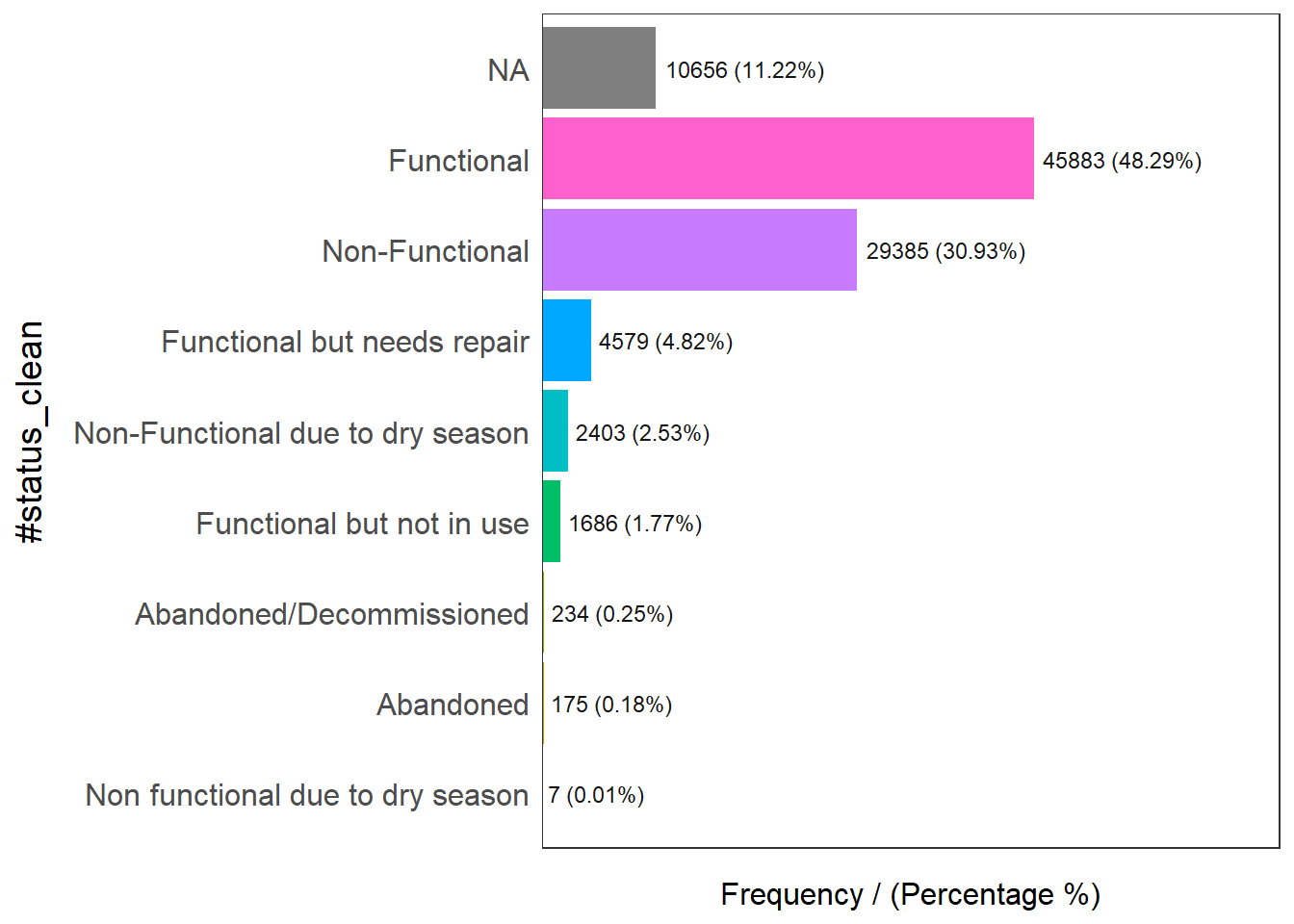

                     #status_clean frequency percentage cumulative_perc
1                       Functional     45883      48.29           48.29
2                   Non-Functional     29385      30.93           79.22
3                             <NA>     10656      11.22           90.44
4      Functional but needs repair      4579       4.82           95.26
5 Non-Functional due to dry season      2403       2.53           97.79
6        Functional but not in use      1686       1.77           99.56
7         Abandoned/Decommissioned       234       0.25           99.81
8                        Abandoned       175       0.18           99.99
9 Non functional due to dry season         7       0.01          100.00

Rename columns

Rename NA so we can do mathematical calculations.

rename() - Remove “#”, for example from ‘#status_clean’ to status_clean for easier handling in subsequent steps.
select () - To select the column status_clean in the output of the sf dataframe.
mutate() & replace_na() to recode all the NA values in status_clean into ‘unknown’

wp_sf_nga <- wp_sf %>%
  rename(status_clean = '#status_clean') %>%
  select(status_clean) %>%
  mutate(status_clean = replace_na(
    status_clean, "unknown"
  ))

Extracting Water Point Data

The code chunk below is used to extract functional water points.

wp_functional <- wp_sf_nga %>% 
  filter(status_clean %in% 
           c("Functional",
             "Functional but not in use", 
             "Functional but needs repair"))

Extract non-functional water points:

wp_nonfunctional <- wp_sf_nga %>% 
  filter(status_clean %in%
           c("Abandoned/Decommissioned",
             "Abandoned",
             "Non-Functional due to dry season", 
             "Non-Functional",
             "Non functional due to dry season"))

Extract water points with unknown status:

wp_unknown <- wp_sf_nga %>% 
  filter(status_clean == "unknown")

Point-in-Polygon Count

Identify functional water points in each LGA by using st_intersects() of the sf_package.
Next, use lengths() to calculate the number of functional water points that fall inside each LGA.

NGA_wp <- NGA %>% 
  mutate(`total_wp` = lengths(
    st_intersects(NGA, wp_sf_nga))) %>%
  mutate(`wp_functional` = lengths(
    st_intersects(NGA, wp_functional))) %>%
  mutate(`wp_nonfunctional` = lengths(
    st_intersects(NGA, wp_nonfunctional))) %>%
  mutate(`wp_unknown` = lengths(
    st_intersects(NGA, wp_unknown)))

These 4 new fields (total_wp, wp_functional, wp_nonfunctional, wp_unknown) are created in NGA_wp.

Visualing attributes by using statistical graphs

gglplot2 package is used to reveal the distribution of total water points by LGA in a histrogram.

ggplot(data = NGA_wp,
       aes(x = total_wp)) + 
  geom_histogram(bins=20,
                 color="black",
                 fill="light blue") +
  geom_vline(aes(xintercept=mean(
    total_wp, na.rm=T)),
             color="red", 
             linetype="dashed", 
             size=0.8) +
  ggtitle("Distribution of total water points by LGA") +
  xlab("No. of water points") +
  ylab("No. of\nLGAs") +
  theme(axis.title.y=element_text(angle = 0))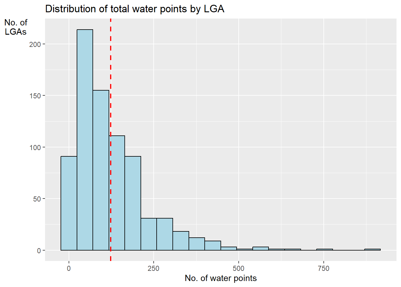

Save the analytical data in rds format

It is recommended retain the sf object structure for subsequent analysis by saving the sf data.frame into rds format.

write_rds(NGA_wp, "data/rds/NGA_wp.rds")